Neuroimaging Analysis Replication and Prediction Study (NARPS)

Here, we specify the statistical model in the NARPS study using a BIDS Stats Model.

The dataset is publicaly available on OpenNeuro.

Setup

%load_ext autoreload
%autoreload 2
import json
from pathlib import Path
from itertools import chain

import numpy as np
import pandas as pd

from nilearn.plotting import plot_design_matrix

import bids
from bids.modeling import BIDSStatsModelsGraph
from bids.layout import BIDSLayout

First, we set up the BIDSLayout object…

layout = BIDSLayout('./ds001734/')

… and load the BIDS Stats Model JSON specification:

json_file = './model-narps_smdl.json'
spec = json.loads(Path(json_file).read_text())
spec

{'Name': 'NARPS',
 'Description': 'NARPS Analysis model',
 'BIDSModelVersion': '1.0.0',
 'Input': {'task': 'MGT'},
 'Nodes': [{'Level': 'Run',
   'Name': 'run',
   'GroupBy': ['run', 'subject'],
   'Transformations': {'Transformer': 'pybids-transforms-v1',
    'Instructions': [{'Name': 'Threshold',
      'Input': ['gain'],
      'Binarize': True,
      'Output': ['trials']},
     {'Name': 'Scale',
      'Input': ['gain', 'loss', 'RT'],
      'Demean': True,
      'Rescale': False,
      'Output': ['gain', 'loss', 'demeaned_RT']},
     {'Name': 'Convolve',
      'Model': 'spm',
      'Input': ['trials', 'gain', 'loss', 'demeaned_RT']}]},
   'Model': {'X': ['trials', 'gain', 'loss', 'demeaned_RT', 1], 'Type': 'glm'},
   'DummyContrasts': {'Contrasts': ['trials', 'gain', 'loss'], 'Test': 't'}},
  {'Level': 'Subject',
   'Name': 'subject',
   'GroupBy': ['subject', 'contrast'],
   'Model': {'X': [1], 'Type': 'meta'},
   'DummyContrasts': {'Test': 't'}},
  {'Level': 'Dataset',
   'Name': 'positive',
   'GroupBy': ['contrast', 'group'],
   'Model': {'X': [1]},
   'DummyContrasts': {'Test': 't'}},
  {'Level': 'Dataset',
   'Name': 'negative-loss',
   'GroupBy': ['contrast', 'group'],
   'Model': {'X': [1]},
   'Contrasts': [{'Name': 'negative',
     'ConditionList': [1],
     'Weights': [-1],
     'Test': 't'}]},
  {'Level': 'Dataset',
   'Name': 'between-groups',
   'GroupBy': ['contrast'],
   'Model': {'X': [1, 'group'], 'Formula': '0 + C(group)'},
   'Contrasts': [{'Name': 'range_vs_indiference',
     'ConditionList': ['C(group)[T.equalRange]',
      'C(group)[T.equalIndifference]'],
     'Weights': [1, -1],
     'Test': 't'}]}],
 'Edges': [{'Source': 'run', 'Destination': 'subject'},
  {'Source': 'subject', 'Destination': 'positive'},
  {'Source': 'subject',
   'Destination': 'negative-loss',
   'Filter': {'contrast': ['loss']}},
  {'Source': 'subject',
   'Destination': 'between-groups',
   'Filter': {'contrast': ['loss']}}]}

Initializing BIDSStatsModelsGraph

Here, we modify the model to restrict it to a single task and three subjects (for demonstration purposes), and initialize the BIDSStatsModelGraph object:

spec['Input'] = {
    'task': 'MGT',
    'subject': ['001']
}

graph = BIDSStatsModelsGraph(layout, spec)

We can visualize the model as a graph:

graph.write_graph()

This graph specifices that a run level model should be run on every subject / run combination, followed by a subject level model, which combines the results of the run level models.

Finally, at the group level, we have three distinct models: a between-group comparison of the ‘loss’ contrast, and within-group one-sample t-tests for the ‘loss’ and ‘positive’ contrasts.

Loading variables

In order to compute the precise design matrices for each level of the model, we need to populate the graph with the specific variables availablet to each Node

Here, we load the BIDSVariableCollection objects, for the entire graph:

try:
    graph.load_collections()
except ValueError:
    graph.load_collections(scan_length=227) # Necessary to define if no BOLD data

Let’s take a look at the variable available at the root run level

root_node = graph.root_node
colls = root_node.get_collections()
colls

[<BIDSRunVariableCollection['RT', 'gain', 'loss', 'participant_response']>,
 <BIDSRunVariableCollection['RT', 'gain', 'loss', 'participant_response']>,
 <BIDSRunVariableCollection['RT', 'gain', 'loss', 'participant_response']>,
 <BIDSRunVariableCollection['RT', 'gain', 'loss', 'participant_response']>]

root_node.group_by

['run', 'subject']

Note that there are multiple instances of the root node, one for each subject / run combination (the node’s group_by is : ['run', 'subject']).

We can access the variables for a specific instance of the root node using variables:

colls[0].variables

{'gain': <SparseRunVariable(name='gain', source='events')>,
 'participant_response': <SparseRunVariable(name='participant_response', source='events')>,
 'RT': <SparseRunVariable(name='RT', source='events')>,
 'loss': <SparseRunVariable(name='loss', source='events')>}

ents = colls[0].entities
print(f"Subject ID: {ents['subject']}, Run ID: {ents['run']}")

Subject ID: 001, Run ID: 1

Executing the graph

Although the graph has defined how Nodes and Edges are linked, and we’ve loaded variables, we need to execute the graph in order to obtain the precise design matrices of each Node.

Executing the graph will begin with the root (in this case run), apply transformations, create a design matrix, and define the node’s outputs as determined by Contrasts. The outputs are then passed via Edges on the subsquent Node, and the process is repetead, until the entire graph is populated

graph.run_graph()

For each instance of the root node, a BIDSStatsModelsNodeOutput object is created, which contains the model specification, and final design matrix for each:

root_node = graph.root_node len(root_node.outputs_)

Run-level Node

Let’s take a look at the first output of the root node (i.e. run level)

first_run = root_node.outputs_[0]

For each, we can access key aspects of the model specification:

first_run.entities

{'run': 1, 'subject': '001'}

# Final design matrix
first_run.X

	trials	gain	loss	demeaned_RT	intercept
0	0.000002	-0.000020	-0.000011	7.939675e-07	1.0
1	-0.000005	0.000056	0.000032	-2.271011e-06	1.0
2	0.000014	-0.000158	-0.000091	6.430126e-06	1.0
3	-0.000037	0.000407	0.000234	-1.652883e-05	1.0
4	0.000073	-0.000810	-0.000466	3.288443e-05	1.0
...	...	...	...	...	...
222	0.580902	1.367049	1.681539	-7.158315e-02	1.0
223	0.565231	3.081296	0.127960	-1.584801e-01	1.0
224	0.617684	5.530195	-1.738936	-2.764609e-01	1.0
225	0.699919	7.956492	-3.449915	-3.903342e-01	1.0
226	0.742641	9.564534	-4.645814	-4.641907e-01	1.0

227 rows × 5 columns

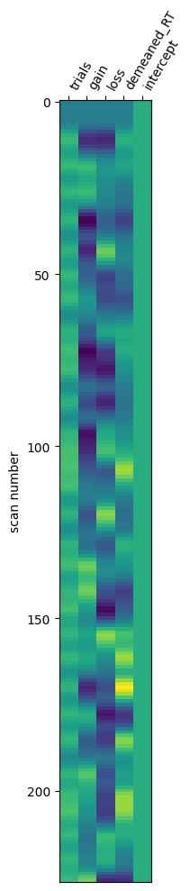
# Plot design matrix
plot_design_matrix(first_run.X)

<Axes: label='conditions', ylabel='scan number'>

The contrasts specify the outputs of the Node that will be passed to subsequent Nodes

# Contrast specification
first_run.contrasts

[ContrastInfo(name='loss', conditions=['loss'], weights=[1], test='t', entities={'run': 1, 'subject': '001', 'contrast': 'loss'}),
 ContrastInfo(name='trials', conditions=['trials'], weights=[1], test='t', entities={'run': 1, 'subject': '001', 'contrast': 'trials'}),
 ContrastInfo(name='gain', conditions=['gain'], weights=[1], test='t', entities={'run': 1, 'subject': '001', 'contrast': 'gain'})]

Subject-level Node

The subject node in this case is a fixed-effects meta-analysis model, which comibines run estimates, separately for each combination of contrast and subject.

We can see how the root node connects to subject, via an Edge:

edge = root_node.children[0]

edge

BIDSStatsModelsEdge(source=<BIDSStatsModelsNode(level=run, name=run)>, destination=<BIDSStatsModelsNode(level=subject, name=subject)>, filter={})

subject_node = edge.destination
subject_node

<BIDSStatsModelsNode(level=subject, name=subject)>

subject_node.level

'subject'

subject_node.group_by

['subject', 'contrast']

Since the subject level Node is group_by : ['subject', 'contrast'], each combination of subject and contrast will have a separate BIDSStatsModelsNodeOutput object:

sub_specs = subject_node.outputs_
sub_specs

[<BIDSStatsModelsNodeOutput(name=subject, entities={'contrast': 'loss', 'subject': '001'})>,
 <BIDSStatsModelsNodeOutput(name=subject, entities={'contrast': 'trials', 'subject': '001'})>,
 <BIDSStatsModelsNodeOutput(name=subject, entities={'contrast': 'gain', 'subject': '001'})>]

Taking a look at a single Nodes’s specification, the design matrix (X) is:

sub_specs[0].X

	intercept
0	1
1	1
2	1
3	1

In this case, we are applying a simple intercept model which is equivalent to a one-sample t-test.

To understand which inputs are associated with this design, we can look at the metadata attribute:

sub_specs[0].metadata

	contrast	run	subject
0	loss	1	001
1	loss	2	001
2	loss	3	001
3	loss	4	001

Finally the contrast for this Node simply passes forward the intercept estimate:

sub_specs[0].contrasts

[ContrastInfo(name='loss', conditions=['intercept'], weights=[1], test='t', entities={'contrast': 'loss', 'subject': '001'})]

Group-level Nodes

Remember that the group-level of this model, we defined three separate Nodes, each performing a different analysis.

• “positive” is a within-group one-sample t-test of all contrasts.

• “negative-loss” is a within-group one-sample t-test for the ‘loss’ contrast, but reversed such that the positive direction is negative.

• “between-groups” is a between-group comparison of the ‘loss’ contrast.

Let’s take a look at each separately:

“Positive” Node (Within-Groups)

Let’s look at the original definition of this Node and the corresponding Edge in the original JSON specification:

spec['Nodes'][3]

{'Level': 'Dataset',
 'Name': 'negative-loss',
 'GroupBy': ['contrast', 'group'],
 'Model': {'X': [1]},
 'Contrasts': [{'Name': 'negative',
   'ConditionList': [1],
   'Weights': [-1],
   'Test': 't'}]}

spec['Edges'][1]

{'Source': 'subject', 'Destination': 'positive'}

This Node specifies to run a separate one-sample t-test for each contrast, for each group separately ('GroupBy': ['contrast', 'group'])

# Run "positive" Node
ds0_node = subject_node.children[0].destination 
ds0_specs = ds0_node.outputs_

ds0_node

<BIDSStatsModelsNode(level=dataset, name=positive)>

There are unique BIDSStatsModelsNodeOutput objects (and thus, models) for each contrast / group combiation:

ds0_specs

[<BIDSStatsModelsNodeOutput(name=positive, entities={'contrast': 'loss', 'group': 'equalIndifference'})>,
 <BIDSStatsModelsNodeOutput(name=positive, entities={'contrast': 'trials', 'group': 'equalIndifference'})>,
 <BIDSStatsModelsNodeOutput(name=positive, entities={'contrast': 'gain', 'group': 'equalIndifference'})>]

Taking a look at this first, we can see the model is a simple intercept model, which is equivalent to a one-sample t-test:

ds0_specs[0].X

	intercept
0	1

With the following inputs:

ds0_specs[0].metadata

	contrast	subject
0	loss	001

“Negative-Loss” Node (Within-Groups)

Next, the “negative-loss” Node takes only the ‘loss’ contrast, and reverses the sign of the positive direction, such that the positive direction is negative.

In the Contrast section of the model, we specify the weight as -1 to flip the sign.

# Negative-loss node specification
spec['Nodes'][4]

{'Level': 'Dataset',
 'Name': 'between-groups',
 'GroupBy': ['contrast'],
 'Model': {'X': [1, 'group'], 'Formula': '0 + C(group)'},
 'Contrasts': [{'Name': 'range_vs_indiference',
   'ConditionList': ['C(group)[T.equalRange]',
    'C(group)[T.equalIndifference]'],
   'Weights': [1, -1],
   'Test': 't'}]}

The corresponding Edge specifies to Filter the input to only include the ‘loss’ contrast:

spec['Edges'][3]

{'Source': 'subject',
 'Destination': 'between-groups',
 'Filter': {'contrast': ['loss']}}

ds1_node = subject_node.children[1].destination
ds1_specs = subject_node.outputs_

The design matrix for the group-level node peforms a simple one-sample t-test on the subject-level contrasts:

ds1_specs[0].X

	intercept
0	1
1	1
2	1
3	1

ds1_specs[0].metadata

	contrast	run	subject
0	loss	1	001
1	loss	2	001
2	loss	3	001
3	loss	4	001

Finally, looking at the contrasts, we can see that the ‘loss’ contrast is passed forward, but with the positive direction flipped:

ds1_specs[0].contrasts

[ContrastInfo(name='loss', conditions=['intercept'], weights=[1], test='t', entities={'contrast': 'loss', 'subject': '001'})]

Between-Groups Node specification

Finally, the “between-groups” Node is a between-group comparison of the ‘loss’ contrast.

Importantly, the GroupBy is set to ['contrast'], such that the model is run separately for each contrast, but the contrasts are combined across groups.

spec['Nodes'][-1]

{'Level': 'Dataset',
 'Name': 'between-groups',
 'GroupBy': ['contrast'],
 'Model': {'X': [1, 'group'], 'Formula': '0 + C(group)'},
 'Contrasts': [{'Name': 'range_vs_indiference',
   'ConditionList': ['C(group)[T.equalRange]',
    'C(group)[T.equalIndifference]'],
   'Weights': [1, -1],
   'Test': 't'}]}

In addition, this Node uses Formula notation to specify the model. The C(group) term specifies a categorical variable, which will be used to specify the between-group comparison.

In the Contrast section, we can refer to specific levels of the categorical variable using the C() notation. Here, we specify a contrast of C(group)[T.equalRange] - C(group)[T.equalIndifference], with weights [1, -1].

As in the previous Node, the corresponding Edge specifies to Filter the input to only include the ‘loss’ contrast:

spec['Edges'][3]

{'Source': 'subject',
 'Destination': 'between-groups',
 'Filter': {'contrast': ['loss']}}

# Get next node from subject
ds2_node = subject_node.children[2].destination 
ds2_specs = ds2_node.outputs_

The design matrix (X) for this Node contrasts subjects 1 and 3 vs 2, as these subjects differ by group:

ds2_specs[0].X

	C(group)[T.equalIndifference]
0	1

ds2_specs[0].metadata

	contrast	subject	suffix
0	loss	001	participants